Logistic Regression
implementation of a logistic regression
Show/Hide the code
| |
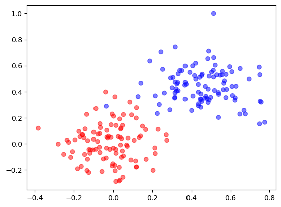
Try Logistic Regression on a Synthetic Dataset
generate data
Show/Hide the code
| |
learn
Show/Hide the code
| |
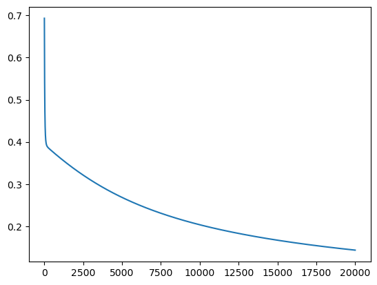
loss
Show/Hide the code
| |
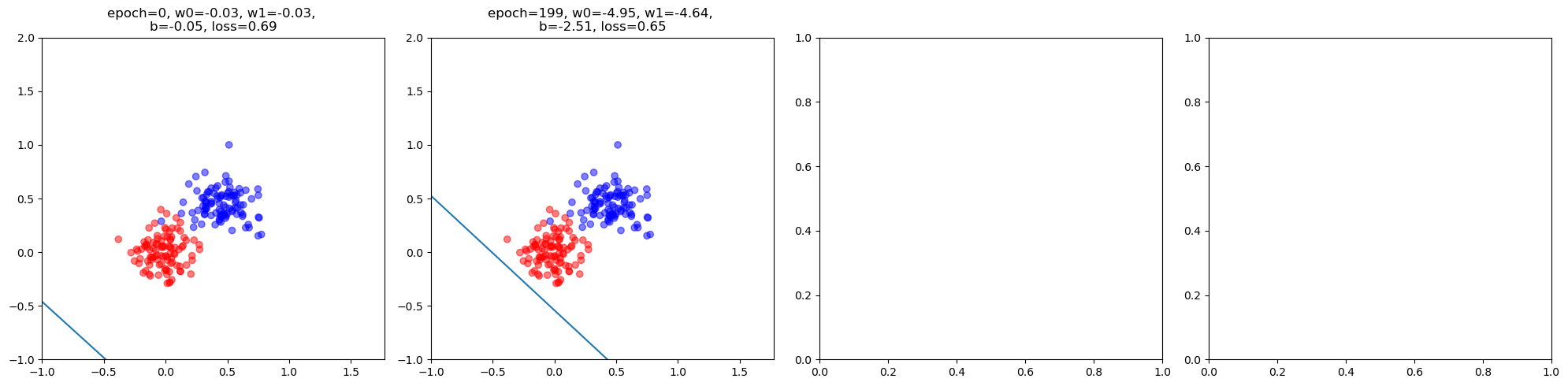
visualize learning process
Show/Hide the code
| |
Try Logistic Regression on a Real Dataset
load data and learn
Show/Hide the code
| |
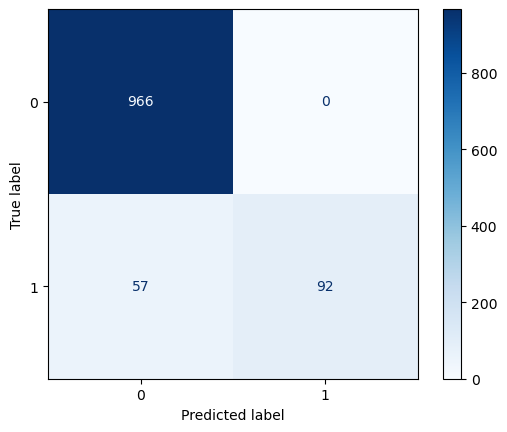
evaluate performance
Show/Hide the code
| |
Accuracy: 0.9488789237668162
Precision: 1.0
Recall: 0.6174496644295302
F1 Score: 0.7634854771784232

Classification Report:

              precision    recall  f1-score   support

         ham       0.94      1.00      0.97       966
        spam       1.00      0.62      0.76       149

    accuracy                           0.95      1115
   macro avg       0.97      0.81      0.87      1115
weighted avg       0.95      0.95      0.94      1115
Show/Hide the code
| |
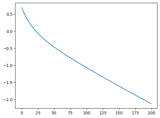
loss
Show/Hide the code
| |