Introduction

Support Vector Machine (SVM), invented by Vladimir Vapnik in 1979, is a kind of machine learning algorithm with solid theoretical foundation (Platt, 1998). The classical implementation of SVM is to find the optimal separating hyperplane by solving a convex quadratic programming problem. Furthermore, by solving its Lagrangian dual problem, kernel methods can be naturally introduced, enabling SVM to handle not only linear classification problems but also complex non-linear ones. This approach primarily uses optimization theory as a tool and can theoretically find an exact analytical solution using Quadratic Programming (QP) solvers. In practice, however, numerical approaches like Sequential Minimal Optimization (SMO) is often employed instead of general QP solvers for better efficiency.

In addition to this perspective, SVM can also be understood from the general machine learning perspective, that is, optimizing a loss function to fit the data. This method typically employs stochastic gradient descent as a tool, gradually approaching the minimum of the loss function by calculating its gradient. The advantage of this method is its simplicity in implementation and lower computational cost, but it usually can only find an approximate solution and cannot utilize kernel methods. The essence of these two methods is the same, just using different viewpoints.

This report will first introduce the linear classification problem and the perceptron algorithm, which is background knowledge and motivation for SVM. Then, the hard margin maximum margin classifier will be introduced in detail, including its primal and lagrange dual form, and an implementation using a QP solver will be provided. The soft margin maximum margin classifier will be presented as an extension to handle noisy and non-linearly separable data. Two implementations of the soft margin classifier will be provided: one using SMO and the other using stochastic gradient descent. These implementations will be compared on both artificial and real-world datasets. Finally, multi-class classification will be discussed, along with a reflection and conclusion of the report.

Links

• GitHub Repository
• Colab Notebook

Background

Linear Classification

SVM is a solution to the linear classification problem. Linear classification refers to the task of classifying data points into different categories based on a linear decision boundary. If the input space \(X\) is a subset of \(\mathbb{R}^n\), where \(n\ge1\) is the number of features in the dataset, a linear decision boundary can be defined as a flat affine subspace of dimension \(n-1\). For example, in a 2-dimensional space, the decision boundary is a line, while in a 3-dimensional space, it is a plane. In higher-dimensional spaces, it is referred to as a hyperplane.

A hyperplane can be defined by the equation:

If a point \(\mathbf{x}_0\) does not lie on the hyperplane, it must either satisfy

or

The side that the point lies on can be determined by its sign:

The learning task of linear classification is to find a hyperplane that separates the data points into two classes correctly, providing the dataset is linearly separable. Therefore, the hypothesis set \(H\) for linear classification can be defined as the set of all possible hyperplanes in the input space \(X\).

Perceptron

Perhaps the simplest algorithm for finding a hyperplane is the Perceptron Learning Algorithm (PLA). The PLA iteratively updates the parameters \(\mathbf{w}\) and \(b\) of the hyperplane based on the misclassified data points. It has been proven that as long as the data is linearly separable, the perceptron algorithm is guaranteed to converge.

Let the class label be denoted by \(y\), where \(y = 1\) for the positive class and \(y = -1\) for the negative class. The product

indicates the correctness of the prediction: a positive value implies a correct prediction, while a negative value indicates a misclassification.

Perceptron learns from misclassifications. When a data point is correctly classified, the algorithm proceeds to the next data point without updating the model, whereas when a data point is misclassified, the model parameters are updated according to the following rules:

where \(lr\) is the learning rate that pre-defined as a hyperparameter.

This update mechanism implies that if the true label is positive and the data point is misclassified, the normal vector \(\mathbf{w}\) of the hyperplane is adjusted in the direction of \(\mathbf{x}\), thereby increasing the likelihood of correctly classifying \(\mathbf{x}\) as a positive instance. Conversely, if the true label is negative, the vector \(\mathbf{w}\) is updated in the opposite direction of \(\mathbf{x}\), making it more likely that \(\mathbf{x}\) will be classified as negative.

 1
 2
 3
 4
 5
 6
 7
 8
 9
10
11
12
13
14
15
16
17
18
19
20
21
22
23
24
25
26
27
28
29
30
31
32
33
34
35
36
37
38
39
40
41
42
43
44

class MyPerceptron:

    def __init__(self, lr=0.1, epochs=10, history=False):
        self.lr = lr
        self.epochs = epochs
        self.history = history
        self.losses = []
        self.records = []

    def f(self, x):
        return x @ self.w + self.b

    def sign(self, x):
        return np.where(x > 0, 1, -1)

    def predict(self, x):
        return self.sign(self.f(x))

    def record(self, w, b, current_loss, i):
        self.records.append([(w, self.w.copy()), (b, self.b), current_loss, i])

    def fit(self, X, y):
        _, n_features = X.shape
        self.w = np.zeros(n_features)
        self.b = 0

        for _ in range(self.epochs):
            for i, (xi, yi) in enumerate(zip(X, y)):
                y_hat = self.predict(xi)

                old_w = self.w.copy()
                old_b = self.b
                if self.history:
                    current_loss = (self.sign(self.f(X)) != y).mean()

                if self.history and current_loss == 0:
                    self.record(old_w, old_b, current_loss, i)
                    return

                if yi * y_hat < 0:
                    self.w += self.lr * yi * xi
                    self.b += self.lr * yi
                    if self.history:
                        self.record(old_w, old_b, current_loss, i)

  1
  2
  3
  4
  5
  6
  7
  8
  9
 10
 11
 12
 13
 14
 15
 16
 17
 18
 19
 20
 21
 22
 23
 24
 25
 26
 27
 28
 29
 30
 31
 32
 33
 34
 35
 36
 37
 38
 39
 40
 41
 42
 43
 44
 45
 46
 47
 48
 49
 50
 51
 52
 53
 54
 55
 56
 57
 58
 59
 60
 61
 62
 63
 64
 65
 66
 67
 68
 69
 70
 71
 72
 73
 74
 75
 76
 77
 78
 79
 80
 81
 82
 83
 84
 85
 86
 87
 88
 89
 90
 91
 92
 93
 94
 95
 96
 97
 98
 99
100
101
102
103

def plot_records(X, y, records, show_legend=True, show_previous=True, figsize=(15, 15)):
    n_updates = len(records)

    cols = 3
    rows = int(np.ceil(n_updates / cols))
    _, axs = plt.subplots(rows, cols, figsize=figsize)
    axs = axs.flatten() if n_updates > 1 else [axs]

    x_margin = 2.0
    y_margin = 2.0
    x_min = np.min(X[:, 0]) - x_margin
    x_max = np.max(X[:, 0]) + x_margin
    y_min = np.min(X[:, 1]) - y_margin
    y_max = np.max(X[:, 1]) + y_margin

    for i in range(n_updates):
        ax = axs[i]
        old_w, new_w = records[i][0]
        old_b, new_b = records[i][1]

        pos_idx = y == 1
        neg_idx = y == -1
        ax.scatter(
            X[pos_idx, 0],
            X[pos_idx, 1],
            color="blue",
            alpha=0.6,
            marker="+",
        )
        ax.scatter(
            X[neg_idx, 0],
            X[neg_idx, 1],
            color="red",
            alpha=0.6,
        )

        ax.scatter(
            X[records[i][3], 0],
            X[records[i][3], 1],
            facecolor="yellow",
            edgecolor="black",
            label="Current Point",
        )

        def plot_hp(w, b, color, linestyle, label):
            x_vals = np.linspace(x_min, x_max, 100)
            if abs(w[1]) > 1e-6:
                y_vals = (-w[0] * x_vals - b) / w[1]
                ax.plot(
                    x_vals,
                    y_vals,
                    color=color,
                    linestyle=linestyle,
                    label=label,
                )
            else:
                x_val = -b / w[0] if abs(w[0]) > 1e-6 else 0
                ax.axvline(x_val, color=color, linestyle=linestyle, label=label)
            return x_vals, y_vals if abs(w[1]) > 1e-6 else None

        plot_hp(new_w, new_b, "black", "-", "After Update")

        if show_previous:
            plot_hp(old_w, old_b, "green", "--", "Before Update")
            x0 = 0
            y0 = (-old_w[0] * x0 - old_b) / old_w[1] if old_w[1] != 0 else 0
            norm = np.linalg.norm(old_w)
            if norm != 0:
                ax.arrow(
                    x0,
                    y0,
                    old_w[0] / norm,
                    old_w[1] / norm,
                    head_width=0.5,
                    width=0.1,
                    color="green",
                )
        x0 = 0
        y0 = (-new_w[0] * x0 - new_b) / new_w[1] if new_w[1] != 0 else 0
        norm = np.linalg.norm(new_w)
        if norm != 0:
            ax.arrow(
                x0,
                y0,
                new_w[0] / norm,
                new_w[1] / norm,
                head_width=0.5,
                width=0.1,
                color="black",
            )

        ax.set_xlim(x_min, x_max)
        ax.set_ylim(y_min, y_max)
        ax.set_title(f"Update {i+1}")
        ax.set_aspect("equal")
        if show_legend:
            ax.legend()

    for j in range(n_updates, len(axs)):
        axs[j].axis("off")

    plt.tight_layout()
    plt.show()

The figure below shows the learning process of a perceptron on a synthetic dataset. The green arrow represents the normal vector before the update, while the black arrow shows the normal vector after the update. For example, in Update 6, when a positive sample (the yellow point) lies on negative side of the hyperplane, the green arrow shifts closer to this data point after the update and thereby the updated hyperplane classifies this point correctly.

1
2
3

perceptron = MyPerceptron(lr=0.1, epochs=2, history=True)
perceptron.fit(X_dummy, y_dummy)
plot_records(X_dummy, y_dummy, perceptron.records[:-1], figsize=(11, 8))

It is clear that after six updates the hyperplane that the perceptron found has separated all data points correctly, but is it the best one? Actually, it is almost the worst, since it is very close to one side. Intuitively, the optimal hyperplane should look like the one below, which maximizes the distance to the nearest data points from both classes. Therefore, the model has a bigger cushion to tolerate noise and outliers. This is the main idea and motivation of SVMs.

 1
 2
 3
 4
 5
 6
 7
 8
 9
10

plt.figure(figsize=(3, 3))
plt.scatter(d1[0:, 0], d1[0:, 1], color="blue", marker="+")
plt.scatter(d2[0:, 0], d2[0:, 1], color="red", marker="o")
plt.plot(
    np.linspace(-2, 6, 10),
    -np.linspace(-2, 6, 10) + 4.1,
    color="black",
)
plt.gca().set_aspect("equal")
plt.show()

Furthermore, the hyperplane found by the perceptron is not unique. Different initializations of the model parameters or variations in the order of data presentation can lead to different hyperplanes (Bishop, 2006). The following figure illustrates six different hyperplanes obtained by perceptron with different shuffles of the training data. Obviously, they vary significantly.

 1
 2
 3
 4
 5
 6
 7
 8
 9
10
11
12
13
14
15
16

params = []
for i in range(6):
    idx = np.random.permutation(len(X_dummy))
    X_shuffled = X_dummy[idx]
    y_shuffled = y_dummy[idx]
    perceptron = MyPerceptron(lr=1, epochs=5, history=True)
    perceptron.fit(X_shuffled, y_shuffled)
    params.append(perceptron.records[-1])
plot_records(
    X_shuffled,
    y_shuffled,
    params,
    show_legend=False,
    show_previous=False,
    figsize=(10, 7),
)

Maximum Margin Classifier With Hard Margin

Maximum Margin Classifier is a solution to the problems of perceptron mentioned above. Unlike Perceptron, Maximum Margin Classifier is able to find the optimal decision boundary by maximizing its margin. Margin is defined to be the smallest distance between the decision boundary and any of the samples (Bishop, 2006).

Functional Distance and Geometric Distance

The distance from a point \(\mathbf{x}_0\) to a hyperplane \(h\) can be calculated by substituting \(\mathbf{x}\) into the equation of the hyperplane:

if the hyperplane correctly classifies the point, the distance can also be expressed as:

where \(y_0\) is the class label of \(\mathbf{x}_0\). This is called the functional distance.

In addition, this value can by manipulated arbitrarily. For example,

represent the same hyperplane, but for the same input \(x\), they yield different values. In fact, the latter is exactly twice the former. Therefore, we can pick a particular scalar to rescale the hyperplane, making it yield preferred output. We choose the scalar to be \(1/\rho\), where

so that:

Therefore, for any hyperplane, we can always rescale it to make the functional distance of the closest data points equal to 1.

Furthermore, the geometric distance from a point \(\mathbf{x}_0\) to the hyperplane \(h_0\) can be calculated as:

In other words, it is the functional distance divided by the norm of the normal vector \(\mathbf{w}\). Geometric distance is also called Euclidean distance, which is invariant to the rescaling of the hyperplane.

The margin of a hyperplane is defined as the geometric distance from the hyperplane to the closest data points. The optimal hyperplane is the one that maximizes the margin. Since the hyperplane is determined by \(\mathbf{w}\) and \(b\), the optimization problem can be formulated as follows:

Since we can always rescale the hyperplane so that

Thus, the optimization problem can be rewritten in a simpler form:

Here, the coefficient \(\frac{1}{2}\) is introduced to simplify the result after differentiation.

Primal Problem

The lagrange function of this optimization problem is:

where \(\alpha_i\ge0\) are the lagrange multipliers.

If we maximize \(L\) w.r.t. \(\alpha\):

It turns out that if there is an \(\mathbf{x}_i\) that satisfies

which violates the constraint, \(L\) will go to \(+\infty\), by making \(\alpha = +\infty\), whereas if all \(\mathbf{x}_i\) satisfy the constraint, the maximum value of \(L\) would be \(\frac{1}{2}||\mathbf{w}||^2\) because we have to make all \(\alpha_i=0\) to avoid negative value.

Therefore, \(\theta(\mathbf{w}, b)\) is actually defined by:

Minimize function \(\theta(\mathbf{w}, b)\) w.r.t. \(\mathbf{w}\) and \(b\):

is equivalent to the original optimization problem and it’s called the primal problem.

Dual Problem

If we instead minimize \(L\) w.r.t. \(\mathbf{w}\) and \(b\) first and then maximize it w.r.t. \(\alpha\), it yields the dual problem:

There are several advantages of solving the dual problem instead of the primal one. First, the dual problem is always a convex optimization problem by nature (this is because the target function is linear w.r.t. \(\alpha\) and the constraint sets are always convex sets), whereas the primal problem may not be convex, though in this case it is. Nevertheless, it’s still a good practice to solve the dual problem, because it is usually simpler to solve than the primal one. It has been proven that for SVMs, solving the dual problem is equivalent to solving the primal one.

To solve the dual problem, first set the derivatives of \(L\) w.r.t. \(\mathbf{w}\) and \(b\) to zero:

we obtain:

substituting them back into \(L\):

Having done that, maximizing w.r.t. \(\alpha\), dual optimization problem can then be summarized as:

Solving the Dual Problem Using a QP Solver

Equation 2 is a simpler quadratic programming problem, which can be solved by standard optimization tools. In this case, cvxopt is used and the standard form of a quadratic programming problem that cvxopt uses is:

To write the dual problem in that form, note that

can be expressed as a quadratic form: \(\alpha^\top P \alpha\), where

Let

where \(I\) is the \(n\times n\) identity matrix. In this way, the dual problem can be written in the standard quadratic programming form:

The corresponding Python code is as follows:

1
2
3
4
5
6

P = matrix(np.outer(y, y) * (X @ X.T))
q = matrix(-np.ones(n_samples))
G = matrix(-np.eye(n_samples))
h = matrix(np.zeros(n_samples))
A = matrix(y.reshape(1, -1).astype(float))
b_eq = matrix(0.0)

After solving for the optimal solution \(\alpha^*\), we can obtain the optimal solution \(\mathbf{w}^*\) and \(b^*\) of the primal problem according to Equation 1 and the Karush-Kuhn-Tucker (KKT) conditions, which are necessary and sufficient conditions for optimality (Platt, 1998):

where \(\mathbf{x}_j\) is any of the support vectors that satisfy \(\alpha^*_j>0\). Here, according to complementary slackness in KKT, \(\alpha_j^*>0\) indicates that \(\mathbf{x}_j\) is a support vector, which lies on the margin boundary and satisfies:

The other data points with \(\alpha_i^*=0\) do not contribute to the decision function, which reveals that the hyperplane depends only on the support vectors.

A better approach to compute \(b\) is to use all support vectors, as this makes it numerically more stable (Bishop, 2006):

where \(S\) is the set of indexes of all support vectors and \(N\) is the number of support vectors.

The Python code for computing \(\mathbf{w}\) and \(b\) based on \(\alpha\) is as follows:

1
2
3
4
5
6

w = np.sum((alphas * labels).reshape(-1, 1) * support_vectors,axis=0)
b = labels[0] - (support_vectors[0] @ w) # use one support vector
b = np.mean([y_i - np.sum(alphas * labels * (X @ x_i)) for i, x_i, y_i in zip(sv_indices, support_vectors, support_vector_labels)]) # use all support vectors

def predict(self, X):
    return np.sign(X @ w + b)

The decision function of the maximum margin classifier is:

or equivalently:

This is because only support vectors have non-zero \(\alpha_i^*\).

 1
 2
 3
 4
 5
 6
 7
 8
 9
10
11
12
13
14
15
16
17
18
19
20
21
22
23
24
25
26
27
28
29
30
31
32
33
34
35
36
37
38
39
40
41
42
43
44
45
46
47
48
49
50
51
52
53
54
55
56
57

import cvxopt
from cvxopt import matrix, solvers


class HardMarginSVM:
    def __init__(self):
        self.w = None
        self.b = None
        self.support_vectors = None
        self.support_vector_labels = None
        self.alphas = None

    def fit(self, X, y):
        n_samples, _ = X.shape

        P = matrix(np.outer(y, y) * (X @ X.T))

        q = matrix(-np.ones(n_samples))

        G = matrix(-np.eye(n_samples))
        h = matrix(np.zeros(n_samples))

        A = matrix(y.reshape(1, -1).astype(float))
        b_eq = matrix(0.0)

        # Solve the quadratic programming problem
        solvers.options["show_progress"] = False
        solution = solvers.qp(P, q, G, h, A, b_eq)

        # Extract alphas
        alphas = np.array(solution["x"]).flatten()

        # Find support vectors (alphas > threshold)
        sv_threshold = 1e-5
        sv_indices = alphas > sv_threshold

        self.support_vectors = X[sv_indices]
        self.support_vector_labels = y[sv_indices]
        self.alphas = alphas[sv_indices]

        # Calculate w
        self.w = np.sum(
            (self.alphas * self.support_vector_labels).reshape(-1, 1)
            * self.support_vectors,
            axis=0,
        )

        # Calculate b using any support vector
        self.b = self.support_vector_labels[0] - np.dot(self.support_vectors[0], self.w)

        return self

    def predict(self, X):
        return np.sign(self.decision_function(X))

    def decision_function(self, X):
        return X @ self.w + self.b

The figure below shows the decision boundary found by the maximum margin classifier on the same synthetic dataset as perceptron used. It is clear that the hyperplane maximizes the margin and classifies all data points correctly.

1
2
3
4
5

qp_svm = HardMarginSVM()
qp_svm.fit(X_dummy, y_dummy)
plt.figure(figsize=(3, 3))
plt.scatter(X_dummy[:, 0], X_dummy[:, 1], c=y_dummy, cmap="bwr", alpha=1)
show_hyperplane(qp_svm.decision_function, (-2, 6))

Maximum Margin Classifier With Soft Margin

Even though a maximum margin classifier is able to find the optimal hyperplane for linearly separable data already, it is quite sensitive to noise and outliers. In addition, real-world data is often not linearly separable, in which case the maximum margin classifier fails to find a decision boundary.

A solution to these problems is to introduce slack variables \(\xi = \{\xi_1, \cdots, \xi_n\}\) for each data point that allow some points to violate the margin or even the decision boundary. In this way, the model gives up classifying all training data correctly, but it allows some data points, which are probably noises or outliers, to be very close to the decision boundary or even on the wrong side of it.

This will increase the bias of the model but reduce its variance, leading to a worse performance on training set, but probably a better performance on testing data. In other words, it generalizes better. Moreover, to trade off the margin size and the number of misclassifications, a regularization parameter \(C\) is introduced. Accordingly, the optimization problem becomes:

and its dual problem becomes:

It turns out that the only difference from the hard margin SVM is that \(\alpha_i\) now has an upper bound \(C\). In addition, the support vectors can be categorized into two types: the first type are those that lie exactly on the margin boundary, which satisfy \(0 < \alpha_i < C\); the second type are those that violate the margin or even the decision boundary, which satisfy \(\alpha_i = C\). The other data points with \(\alpha_i = 0\) still do not contribute to the decision function.

Sequential Minimal Optimization

Sequential Minimal Optimization (SMO) is a popular algorithm for solving the dual problem of the soft margin SVM. The main idea behind SMO is coordinate descent optimized specifically for the SVM dual problem. Coordinate descent refers to optimizing one variable at a time while keeping the others fixed. Therefore, for convex optimization problems, the optimization problem is reduced to finding the minimum of a single variable convex function. However, in the case of SVM dual problem, there is an equality constraint:

for which if we optimize one \(\alpha_i\) at a time, it is impossible to satisfy the constraint. To address this issue, SMO optimizes two variables at a time, which allows to adjust one variable while compensating with the other to satisfy the equality constraint.

The following conclusions are from Platt (1998).

Two-variable Optimization

According to Equation 1, we have:

Let \(E_i = f(\mathbf{x}_i) - y_i\) and \(K_{ij} = \mathbf{x}_i \cdot \mathbf{x}_j\).

Assuming we select \(\alpha_1\) and \(\alpha_2\) to optimize, the unclipped solution is:

where \(\eta = 2K_{12} - K_{11} - K_{22}\).

To ensure that the new \(\alpha_1\) and \(\alpha_2\) satisfy the constraints, we need to clip them within the feasible region. The clipping bounds depend on whether \(y_1\) and \(y_2\) are the same or different:

The pseudo Python code below demonstrates the two-variable optimization process. i1, i2 are the indexes of the two variables being optimized. The array alphas stores the values of all \(\alpha_i\) and y stores the class labels. The function compute_error computes the error \(E_i\), which is the difference between the predicted and true labels. The code first ensures that the two selected variables are different and initializes the necessary variables.

1
2
3
4

if i1 == i2: return 0
alpha1, alpha2 = alphas[i1], alphas[i2]
y1, y2 = y[i1], y[i2]
E1, E2 = compute_error(i1), compute_error(i2)

Then, it calculates the bounds \(L\) and \(H\) for clipping based on the conclusions Equation 4 and ensures \(L \ne H\).

1
2
3
4
5
6
7
8

s = y1 * y2
if y1 != y2:
    L = max(0, alpha2 - alpha1)
    H = min(self.C, self.C + alpha2 - alpha1)
else:
    L = max(0, alpha1 + alpha2 - self.C)
    H = min(self.C, alpha1 + alpha2)
if L == H: return 0

K is the kernel matrix (Since the kernel trick has not been introduced, it is just the inner product of vectors here). The code finally computes the new values of \(\alpha_2\), clips \(\alpha_2\) within the bounds \(L\) and \(H\), and updates \(\alpha_1\) accordingly, based on Equation 3.

1
2
3
4
5
6
7
8
9

k11, k12, k22 = K[i1, i1], K[i1, i2], K[i2, i2]
eta = k11 + k22 - 2 * k12
if eta > 0:
    alpha2_new = alpha2 + y2 * (E1 - E2) / eta
    if alpha2_new >= H: alpha2_new = H
    elif alpha2_new <= L: alpha2_new = L
else:
    alpha2_new = L if abs(alpha2 - L) < abs(alpha2 - H) else H
alpha1_new = alpha1 + s * (alpha2 - alpha2_new)

Choosing Variables

In fact, as long as SMO always selects two variables to optimize, it will eventually converge (Platt, 1998). To speed up this process, SMO uses heuristics to choose variables. The selections of the first and the second variable are called the outer and inner loop, respectively.

According to Platt (1998), the algorithm for selecting two variables is as follows:

Outer Loop:

1. Iterates over all data points and examines whether they violate the KKT conditions. If a data point violates the KKT conditions, it is eligible for selection.
2. Iterate only over non-bound examples (\(0 < \alpha < C\))
3. Repeat step 2 until all of the non-bound examples obey the KKT conditions within a specified tolerance, typically \(10^{-3}\).
4. Alternate between “entire training set pass” and “repeated non-bound subset passes” until entire training set satisfies KKT conditions.

Inner Loop:

1. Approximate step size by \(|E_1 - E_2|\). If \(E_i > 0\), choose example with minimum \(E_2\), whereas if \(E_1 < 0\): choose example with maximum \(E_2\).

If the choice of the second variable makes no positive progress, then iterate through non-bound examples, and find one that makes positive progress; If still no progress, iterate through entire training set. If nothing works, skip this pair and return to the outer loop.

Computing \(b\)

1. If \(\alpha_1\) is non-bound: use \(b_1\)
2. If \(\alpha_2\) is non-bound: use \(b_2\)
3. If both non-bound: use either (they should be equal, or average for numerical stability)
4. If both bound: use \(\frac{(b_1 + b_2)}{2}\)

  1
  2
  3
  4
  5
  6
  7
  8
  9
 10
 11
 12
 13
 14
 15
 16
 17
 18
 19
 20
 21
 22
 23
 24
 25
 26
 27
 28
 29
 30
 31
 32
 33
 34
 35
 36
 37
 38
 39
 40
 41
 42
 43
 44
 45
 46
 47
 48
 49
 50
 51
 52
 53
 54
 55
 56
 57
 58
 59
 60
 61
 62
 63
 64
 65
 66
 67
 68
 69
 70
 71
 72
 73
 74
 75
 76
 77
 78
 79
 80
 81
 82
 83
 84
 85
 86
 87
 88
 89
 90
 91
 92
 93
 94
 95
 96
 97
 98
 99
100
101
102
103
104
105
106
107
108
109
110
111
112
113
114
115
116
117
118
119
120
121
122
123
124
125
126
127
128
129
130
131
132
133
134
135
136
137
138
139
140
141
142
143
144
145
146
147
148
149
150
151
152
153
154
155
156
157
158
159
160
161
162
163
164
165
166
167
168
169
170
171
172
173
174
175
176
177
178
179
180
181
182
183
184
185
186
187
188
189

## | echo: false
class SMOSVM:
    def __init__(self, C=1.0, tol=1e-3, max_iter=100, gamma=1.0):
        self.C = C
        self.tol = tol
        self.max_iter = max_iter

    def _compute_error(self, i):
        return self.f[i] - self.y[i]

    def _take_step(self, i1, i2):
        if i1 == i2:
            return 0

        alpha1 = self.alphas[i1]
        alpha2 = self.alphas[i2]
        y1 = self.y[i1]
        y2 = self.y[i2]
        E1 = self._compute_error(i1)
        E2 = self._compute_error(i2)
        s = y1 * y2

        if y1 != y2:
            L = max(0, alpha2 - alpha1)
            H = min(self.C, self.C + alpha2 - alpha1)
        else:
            L = max(0, alpha1 + alpha2 - self.C)
            H = min(self.C, alpha1 + alpha2)

        if L == H:
            return 0

        k11 = self.K[i1, i1]
        k12 = self.K[i1, i2]
        k22 = self.K[i2, i2]
        eta = k11 + k22 - 2 * k12

        if eta > 0:
            alpha2_new = alpha2 + y2 * (E1 - E2) / eta

            if alpha2_new >= H:
                alpha2_new = H
            elif alpha2_new <= L:
                alpha2_new = L
        else:
            alpha2_new = L if abs(alpha2 - L) < abs(alpha2 - H) else H

        if abs(alpha2_new - alpha2) < 1e-5:
            return 0

        alpha1_new = alpha1 + s * (alpha2 - alpha2_new)

        b1 = (
            self.b
            - E1
            - y1 * (alpha1_new - alpha1) * k11
            - y2 * (alpha2_new - alpha2) * k12
        )
        b2 = (
            self.b
            - E2
            - y1 * (alpha1_new - alpha1) * k12
            - y2 * (alpha2_new - alpha2) * k22
        )

        if 0 < alpha1_new < self.C:
            b_new = b1
        elif 0 < alpha2_new < self.C:
            b_new = b2
        else:
            b_new = (b1 + b2) / 2

        self.alphas[i1] = alpha1_new
        self.alphas[i2] = alpha2_new
        self.b = b_new

        self.f = np.sum(self.alphas * self.y * self.K.T, axis=1) + self.b

        return 1

    # pick up i1 and run the optimization process
    def _examine_example(self, i2):
        y2 = self.y[i2]
        alpha2 = self.alphas[i2]
        E2 = self._compute_error(i2)

        # E = (f-y) => r = y*f - y*y = y*f - 1 = functional distance - 1
        r2 = E2 * y2

        # two cases of violating KKT
        # r < 0 => functional distance < 1, alpha should be C but < C
        # r > 0 => functional distance > 1, alpha should be 0 but > 0
        if (r2 < -self.tol and alpha2 < self.C) or (r2 > self.tol and alpha2 > 0):

            # 0 < alphas < C => points lay exactly on the margin
            non_bound_indices = np.where((self.alphas > 0) & (self.alphas < self.C))[0]

            # if there are at least another one non-bound alpha
            if len(non_bound_indices) > 1:
                errors = np.array([self._compute_error(i) for i in non_bound_indices])
                if E2 > 0:
                    i1 = non_bound_indices[np.argmin(errors)]
                else:
                    i1 = non_bound_indices[np.argmax(errors)]

                if self._take_step(i1, i2):
                    return 1

                # if heuristic does not work, try to pick one randomly
                np.random.shuffle(non_bound_indices)
                for i1 in non_bound_indices:
                    if self._take_step(i1, i2):
                        return 1
            # if nothing works or there is only one non-bound alpha
            all_indices = np.random.permutation(self.n)
            for i1 in all_indices:
                if self._take_step(i1, i2):
                    return 1

        return 0

    def _compute_kernel_matrix(self, X):
        return X @ X.T

    def fit(self, X, y):
        self.X = X
        self.y = y
        self.n, self.d = X.shape

        # initialize alphas, 0 <= alphas <= C
        self.alphas = np.zeros(self.n)
        self.b = 0.0

        self.K = self._compute_kernel_matrix(X)

        self.f = np.zeros(self.n) + self.b

        num_changed = 0
        examine_all = True
        iter_count = 0

        # as long as:
        # 1. there are alphas have been updated or
        # 2. we try to examine all alphas or
        # 3. we haven't reached the limitation
        # try to pick up two alphas to optimize
        while (num_changed > 0 or examine_all) and iter_count < self.max_iter:
            num_changed = 0

            if examine_all:
                # i2 would be any alphas
                for i in range(self.n):
                    num_changed += self._examine_example(i)
            else:
                non_bound_indices = np.where(
                    (self.alphas > 0) & (self.alphas < self.C)
                )[0]
                for i in non_bound_indices:
                    num_changed += self._examine_example(i)

            # if we just done examine all alphas, next time try non-bound alphas only
            if examine_all:
                examine_all = False
            # otherwise, if non-bound alphas do not work, we try to examine all next time
            elif num_changed == 0:
                examine_all = True

            iter_count += 1

        sv_indices = self.alphas > 1e-5
        self.support_vectors_ = X[sv_indices]
        self.support_vector_labels_ = y[sv_indices]
        self.support_vector_alphas_ = self.alphas[sv_indices]

    def decision_function(self, X):
        n_samples = X.shape[0]
        decision = np.zeros(n_samples)

        for i in range(n_samples):
            K = (X[i : i + 1] @ self.support_vectors_.T).flatten()
            decision[i] = (
                np.sum(self.support_vector_alphas_ * self.support_vector_labels_ * K)
                + self.b
            )

        return decision

    def predict(self, X):
        return np.sign(self.decision_function(X))

The figure below shows the decision boundary found by SMO SVM on a noisy dataset. It can be seen that the hyperplane allows some points to violate the margin and even be misclassified.

 1
 2
 3
 4
 5
 6
 7
 8
 9
10
11
12

smo_svm = SMOSVM(C=0.2, tol=1e-3, max_iter=100)
smo_svm.fit(X_with_noise, y_with_noise)

# Plot the decision boundary
plt.figure(figsize=(3, 3))
plt.scatter(
    X_with_noise[:, 0], X_with_noise[:, 1], c=y_with_noise, cmap="bwr", alpha=0.6, s=100
)

show_hyperplane(smo_svm.decision_function)

plt.show()

Hinge Loss With L2 Regularization

In addition to solving the dual problem, the soft margin SVM can also be addressed from another perspective: optimizing the regularized hinge loss. It can be shown that the original optimization problem of the soft margin SVM is equivalent to the following optimization problem:

Here, the first term is the regularization term, and \(\lambda\) is the regularization parameter, which controls the trade-off between the two terms and is inversely proportional to \(C\) above. When \(\lambda\) approaches 0, the penalty from regularization decreases, and the model tends to classify the data correctly. When \(\lambda=0\), the model essentially becomes the hard margin SVM.

In this case, if the dataset is linearly separable, the model can find a hyperplane that perfectly classifies the data, but it will be extremely sensitive to noise and outliers, leading to poor generalization. To balance perfect classification with generalization ability, \(\lambda\) is usually set to a value greater than 0. In this way, while the model pursues perfect classification, it also minimizes the norm of the weights as much as possible, thereby enlarging the margin (recall that the margin is the inverse of \(||\mathbf{w}||\)), and improving generalization.

From the perspective of model complexity, regularization constrains the parameter space by eliminating large values of weights, thus limiting the number of hypotheses in the hypothesis set \(\mathbb{H}\), reducing model complexity, and lowering the risk of overfitting. This reflects the idea of the bias-variance trade-off.

The second term is the hinge loss, which is named after its shape, as shown in the figure below. When the functional margin is greater than or equal to 1

it means the point lies outside the margin or exactly on it, so no penalty is applied. When the margin is less than 1, the penalty equals the distance by which the point falls short of the margin. The closer the point is to the hyperplane, the larger the violation of the margin, and thus the heavier the penalty.

1
2
3
4
5
6
7
8
9

plt.figure(figsize=(4, 2))
xvals = np.linspace(-10, 10, 1000)
yvals = np.maximum(0, 1 - xvals)
plt.plot(xvals, yvals, "b-")
plt.axhline(y=0, color="black", alpha=0.3)
plt.axvline(color="black", alpha=0.3)
plt.xlim(-3, 5)
plt.ylim(-1, 4)
plt.show()

The following code demonstrates how to compute hinge loss with L2 regularization in Python. First, the distance of each point to the hyperplane is calculated. Points with distance greater than 1 are set to 0, and then the average is taken to obtain the hinge loss. The regularization term is computed according to the formula, and finally the two terms are added together to obtain the final loss value.

1
2
3
4
5

def loss(X, y, w, b, lambda_):
    distances = y * (X @ w + b)
    hinge_loss = np.mean(np.maximum(0, 1 - distances))
    reg_loss = lambda_ * (w @ w)
    return hinge_loss + reg_loss

Mini-batch SGD

Since the hinge loss is almost everywhere differentiable and is a convex function, in addition to analytical methods, one can also use stochastic gradient descent (SGD) to find the minimum. SGD refers to updating the parameters in the direction determined by the gradient of the function. At non-differentiable points, a sub-gradient is chosen to replace the gradient. For example, for the hinge loss function, at non-differentiable points, any element from

can be chosen as the sub-gradient. Since the gradient always points in the direction of steepest ascent, its negative points to the steepest descent direction. Because the objective function is convex, descending along the steepest slope at each step will gradually lead us closer to the minimum of the function, i.e., the point where the hinge loss is minimized.

The stochastic nature of SGD comes from computing the gradient on a small randomly sampled batch of data from the dataset each time. This avoids the expensive computation cost of calculating gradients over the entire dataset, while also avoiding the instability of using just a single data point, thus achieving a balance.

Gradient Calculation

To compute the gradient of the hinge loss, first write hinge loss in a piecewise form:

This function is non-differentiable at the piecewise boundary, but differentiable elsewhere. When \(1-y_i(\mathbf{w}\cdot\mathbf{x}_i+b)>0\),

When \(1-y_i(\mathbf{w}\cdot\mathbf{x}_i+b) < 0\), the hinge loss is 0, and only the regularization term is considered:

The following code demonstrates how to compute the gradient. First, the distance of each point to the hyperplane is calculated. Then, depending on whether the distance is greater than 1, the gradient is computed differently. For points with distance less than 1, the gradient is the sum of the hinge loss gradient and the regularization term gradient. For points with distance greater than 1, the hinge loss gradient is 0, and only the regularization term gradient is computed. Here, for points with distance exactly equal to 1, the sub-gradient is chosen to be 0.

 1
 2
 3
 4
 5
 6
 7
 8
 9
10

def calc_gradient(X, y, w, b, lambda_):
    distances = y * (X @ w + b)
    mask = distances < 1
    dw = 2 * lambda_ * w
    if np.any(mask):
        dw += -np.mean((y[mask]).reshape(-1, 1) * X[mask], axis=0)
    db = 0.0
    if np.any(mask):
        db = -np.mean(y[mask])
    return dw, db

Learning Rate

The gradient determines the update direction at each step, while the learning rate controls the step size. If the learning rate is too large, the algorithm may overshoot the minimum, or even cause the loss to increase. If the learning rate is too small, convergence will be very slow, and in the case of non-convex optimization, it may increase the risk of getting stuck in a local optimum. Therefore, choosing an appropriate learning rate is also crucial. The two cases described above are illustrated in the figure below.

 1
 2
 3
 4
 5
 6
 7
 8
 9
10
11
12
13
14
15
16
17
18
19
20
21
22
23
24
25
26
27
28
29
30
31
32
33
34

def f(x):
    return np.array(x) ** 2


fig, axes = plt.subplots(1, 2, figsize=(8, 3))

x = np.linspace(-2, 2, 100)
y = f(x)
axes[0].plot(x, y, "b-")
axes[0].axhline(y=0, color="black", alpha=0.3)
axes[0].axvline(color="black", alpha=0.3)
axes[0].set_ylim(-1, 4)
axes[0].set_xlim(-2, 2)
axes[0].scatter([-1.0], f([-1.0]), color="red")
axes[0].plot([-1.0, 1.5], [f(-1), f(-1)], "r--")
axes[0].axvline(x=1.5, color="black", alpha=0.3, linestyle="--")
axes[0].scatter([1.5], f([1.5]), color="green")
axes[0].text(-1.0, 1.2, "Start", fontsize=10, color="red")
axes[0].text(0.4, 2.3, "Overshoot", fontsize=10, color="green")
axes[0].set_title("Too Large, Loss Increases", fontsize=10)

axes[1].plot(x, y, "b-")
axes[1].axhline(y=0, color="black", alpha=0.3)
axes[1].axvline(color="black", alpha=0.3)
axes[1].set_ylim(-1, 4)
axes[1].set_xlim(-2, 2)
axes[1].scatter([-1.8], f([-1.8]), color="red")
axes[1].plot([-1.8, -1.7], [f(-1.8), f(-1.8)], "r--")
axes[1].axvline(x=-1.7, color="black", alpha=0.3, linestyle="--")
axes[1].scatter([-1.7], f([-1.7]), color="green")
axes[1].text(-1.6, 3.3, "Start", fontsize=10, color="red")
axes[1].text(-1.5, 2.7, "Too slow", fontsize=10, color="green")
axes[1].set_title("Too Small, Loss Decreases Slowly", fontsize=10)
plt.show()

Apart from using a fixed learning rate, a dynamically adjusted learning rate can be used. For example, the learning rate can gradually decrease as the number of iterations increases. The advantage of this approach is that in the initial stage, a larger learning rate allows the algorithm to quickly approach the optimal solution; while in the later stage, a smaller learning rate helps avoid overshooting the optimum and allows more stable convergence.

Update Strategy

Having calculated the gradient and chosen a appropriate learning rate, the parameters can be updated as follows:

where \(lr\) is the learning rate.

The complete learning process is as follows:

1. First, randomly initialize the model parameters \(\mathbf{w}\) and \(b\).
2. Then, in each iteration, split all the data into multiple mini-batches.
3. For each mini-batch, compute the gradient for that batch and update the model parameters.
4. Repeat steps 2 and 3 until the preset number of iterations is reached.

The code is shown below:

1
2
3
4
5
6
7
8
9

w = np.random.normal(0, 0.01, n_features)
b = 0.0

for epoch in range(n_epochs):
    batches = get_batches(X, y, batch_size)
    for batch in batches:
        dw, db = gradient(X_batch, y_batch)
        w -= lr * dw
        b -= lr * db

 1
 2
 3
 4
 5
 6
 7
 8
 9
10
11
12
13
14
15
16
17
18
19
20
21
22
23
24
25
26
27
28
29
30
31
32
33
34
35
36
37
38
39
40
41
42
43
44
45
46
47
48
49
50
51
52
53
54
55
56
57
58
59
60
61
62
63

class SGDSVM:
    def __init__(self, lambda_=0.01, lr=0.01, epochs=10, batch_size=64):
        self.lambda_ = lambda_
        self.lr = lr
        self.epochs = epochs
        self.batch_size = batch_size
        self.loss_history = []

    def loss(self, X, y):
        distances = 1 - y * (X @ self.w + self.b)
        hinge_loss = np.maximum(0, distances).mean()
        reg = self.lambda_ * (self.w @ self.w)
        return hinge_loss + reg

    def gradient(self, X, y):

        # Decision values for batch
        distances = 1 - y * (X @ self.w + self.b)

        # Identify samples with hinge loss > 0
        mask = distances > 0

        # Gradient w.r.t w
        dw = 2 * self.lambda_ * self.w
        if np.any(mask):
            dw += -np.mean((y[mask]).reshape(-1, 1) * X[mask], axis=0)

        # Gradient w.r.t b
        db = 0.0
        if np.any(mask):
            db = -np.mean(y[mask])

        return dw, db

    def fit(self, X, y):
        np.random.seed(42)
        n_samples, n_features = X.shape
        self.w = np.random.normal(0, 0.01, n_features)
        self.b = 0.0

        self.losses_train = []

        for epoch in range(self.epochs):
            indices = np.random.permutation(n_samples)
            X_shuffled, y_shuffled = X[indices], y[indices]

            for i in range(0, n_samples, self.batch_size):

                # numpy array never go out of index range with slicing
                X_batch = X_shuffled[i : i + self.batch_size]
                y_batch = y_shuffled[i : i + self.batch_size]

                dw, db = self.gradient(X_batch, y_batch)
                self.w -= self.lr * dw
                self.b -= self.lr * db

            self.loss_history.append(self.loss(X, y))

    def decision_function(self, X):
        return X @ self.w + self.b

    def predict(self, X):
        return np.sign(self.decision_function(X))

Comparison With Hard Margin SVM

As shown in the figure below, after introducing two outliers into the original dataset, the decision boundary of the hard margin classifier is largely shifted due to the influence of the noise, producing a hyperplane with very narrow margins, whereas the soft margin classifier is less affected by outliers, because it allows some points to violate the margin or even be misclassified.

 1
 2
 3
 4
 5
 6
 7
 8
 9
10
11
12
13
14
15
16
17

hard_svm = HardMarginSVM()
hard_svm.fit(X_with_noise, y_with_noise)
sgd_svm = SGDSVM(epochs=200, lr=0.01, lambda_=0.1)
sgd_svm.fit(X_with_noise, y_with_noise)

fig, axes = plt.subplots(1, 2, figsize=(6, 3))
axes[0].scatter(
    X_with_noise[:, 0], X_with_noise[:, 1], c=y_with_noise, cmap="bwr", alpha=1
)
axes[0].set_title("Hard Margin SVM", fontsize=10)
axes[1].set_title("Soft Margin SVM", fontsize=10)
axes[1].scatter(
    X_with_noise[:, 0], X_with_noise[:, 1], c=y_with_noise, cmap="bwr", alpha=1
)
show_hyperplane(hard_svm.decision_function, ax=axes[0])
show_hyperplane(sgd_svm.decision_function, ax=axes[1])
plt.show()

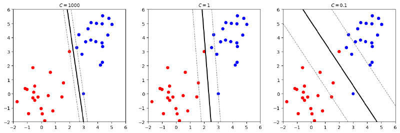
The figure below shows different decision boundaries obtained by the soft margin SVM with different values of the regularization parameter \(\lambda\). A smaller \(\lambda\) (equivalent to a larger \(C\)) means a smaller penalty for misclassification, leading to a narrower margin and a more complex model that fits the training data better but may overfit. Conversely, a larger \(\lambda\) (equivalent to a smaller \(C\)) results in a wider margin and a simpler model that may underfit the training data but generalizes better.

 1
 2
 3
 4
 5
 6
 7
 8
 9
10
11
12

fig, axes = plt.subplots(1, 3, figsize=(15, 5))
Cs = [1000, 1, 0.1]
titles = [r"$C=1000$", r"$C=1$", r"$C=0.1$"]
for ax, C, title in zip(axes, Cs, titles):
    smo_svm = SMOSVM(C, tol=1e-3, max_iter=100)
    smo_svm.fit(X_with_noise, y_with_noise)
    ax.set_title(title, fontsize=10)
    ax.scatter(
        X_with_noise[:, 0], X_with_noise[:, 1], c=y_with_noise, cmap="bwr", alpha=1
    )
    show_hyperplane(smo_svm.decision_function, ax=ax)
plt.show()

Experiments On MNIST Dataset

Dataset Description

The input dataset \(X\) consists of \(28\times28\) pixel grayscale images of handwritten digits. The pixel values range from 0 to 255 where 0 represents pure white and 255 represents pure black. The pixel values are normalized to the range \([0, 1]\) by dividing by 255. The training set contains 60,000 images and the test set contains 10,000 images. In this experiment, only the digits 3 and 7 are used to form a binary classification problem. Each image is flattened into a 784-dimensional vector. The output is a binary label indicating whether the digit is a 3 or a 7.

 1
 2
 3
 4
 5
 6
 7
 8
 9
10
11
12
13
14
15
16
17
18

import idx2numpy

train_images = idx2numpy.convert_from_file("./mnist/archive/train-images.idx3-ubyte")
train_labels = idx2numpy.convert_from_file("./mnist/archive/train-labels.idx1-ubyte")
test_images = idx2numpy.convert_from_file("./mnist/archive/t10k-images.idx3-ubyte")
test_labels = idx2numpy.convert_from_file("./mnist/archive/t10k-labels.idx1-ubyte")
threes = train_images[train_labels == 3].reshape(-1, 28 * 28).astype(np.float32) / 255.0
sevens = train_images[train_labels == 7].reshape(-1, 28 * 28).astype(np.float32) / 255.0
fives = train_images[train_labels == 5].reshape(-1, 28 * 28).astype(np.float32) / 255.0
fives_valid = (
    test_images[test_labels == 5].reshape(-1, 28 * 28).astype(np.float32) / 255.0
)
threes_valid = (
    test_images[test_labels == 3].reshape(-1, 28 * 28).astype(np.float32) / 255.0
)
sevens_valid = (
    test_images[test_labels == 7].reshape(-1, 28 * 28).astype(np.float32) / 255.0
)

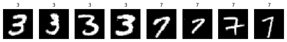
The figure below shows some samples of the digits 3 and 7 from the training set.

 1
 2
 3
 4
 5
 6
 7
 8
 9
10
11
12
13
14
15
16
17
18

X = np.vstack([threes, sevens])
y = np.array([1] * len(threes) + [-1] * len(sevens))
X_valid = np.vstack([threes_valid, sevens_valid])
y_valid = np.array([1] * len(threes_valid) + [-1] * len(sevens_valid))

show_images(
    [
        threes[0].reshape(28, 28),
        threes[1].reshape(28, 28),
        threes[2].reshape(28, 28),
        threes[3].reshape(28, 28),
        sevens[0].reshape(28, 28),
        sevens[1].reshape(28, 28),
        sevens[2].reshape(28, 28),
        sevens[3].reshape(28, 28),
    ],
    titles=["3", "3", "3", "3", "7", "7", "7", "7"],
)

Training with SGD SVM

The code below trains a soft margin SGD based SVM.

1
2

sgd_svm = SGDSVM(epochs=200, lr=0.0001, lambda_=0.001)
sgd_svm.fit(X, y)

The figure below shows the training loss curve. It can be seen that the loss decreases rapidly in the initial stage and then gradually stabilizes.

1
2
3
4
5

plt.figure(figsize=(6, 3))
plt.plot(sgd_svm.loss_history, color="blue", label="Training Loss")

plt.legend()
plt.show()

The code below calculates the accuracy on the validation set.

1
2
3

print(
    f"The accuracy on the validation set is: {(sgd_svm.predict(X_valid) == y_valid).mean()*100:.2f}%"
)

The accuracy on the validation set is: 98.28%

The figure below visualizes the learned weights. The red areas indicate positive weights, while the blue areas indicate negative weights. It can be observed that the model focuses on the regions that are most discriminative between the digits 3 and 7.

1

plt.imshow(sgd_svm.w.reshape(28, 28), cmap="RdBu", aspect="equal")

The figure below shows the confusion matrix of the predictions on the validation set. It can be seen that most samples are correctly classified, with only a few misclassifications.

 1
 2
 3
 4
 5
 6
 7
 8
 9
10
11
12
13
14
15
16
17
18
19

from sklearn.metrics import confusion_matrix, classification_report, accuracy_score
import seaborn as sns

y_pred = sgd_svm.predict(X_valid)

cm = confusion_matrix(y_valid, y_pred)

plt.figure(figsize=(5, 4))
sns.heatmap(
    cm,
    annot=True,
    fmt="d",
    cmap="Blues",
    xticklabels=["7", "3"],
    yticklabels=["7", "3"],
)
plt.xlabel("Predicted")
plt.ylabel("True")
plt.show()

The table below shows the precision, recall, and F1-score for each class.

1

print(classification_report(y_valid, y_pred, target_names=["7", "3"]))

              precision    recall  f1-score   support

           7       0.99      0.98      0.98      1028
           3       0.98      0.99      0.98      1010

    accuracy                           0.98      2038
   macro avg       0.98      0.98      0.98      2038
weighted avg       0.98      0.98      0.98      2038

Comparison with SMO Algorithm

SMO algorithm is expected to be able to find a more accurate solution to the soft margin SVM problem because it directly solves the dual problem. The code below randomly selects 500 samples from the training set to form a smaller training set and trains an SMO SVM on it.

1
2
3
4
5
6
7

n_train_samples = 500
indices = np.random.choice(len(X), n_train_samples, replace=False)
X_train_small = X[indices]
y_train_small = y[indices]

smo_mnist = SMOSVM(C=100, tol=1e-3, max_iter=50)
smo_mnist.fit(X_train_small, y_train_small)

The code below evaluates the SMO SVM on the validation set and compares it with the SGD SVM trained on the same small subset. SMO SVM and SGD SVM have almost the same performance.

 1
 2
 3
 4
 5
 6
 7
 8
 9
10

## Evaluate SMO SVM on validation set
y_pred_smo = smo_mnist.predict(X_valid)
accuracy_smo = accuracy_score(y_valid, y_pred_smo)
print(f"SMO SVM accuracy on validation set: {accuracy_smo*100:.2f}%")

sgd_svm_small = SGDSVM(epochs=1000, lr=0.0001, lambda_=0.001)
sgd_svm_small.fit(X_train_small, y_train_small)
y_pred_sgd_small = sgd_svm_small.predict(X_valid)
accuracy_sgd_small = accuracy_score(y_valid, y_pred_sgd_small)
print(f"SGD SVM accuracy on validation set: {accuracy_sgd_small*100:.2f}%")

References

Bishop, C. M. (2006). Pattern recognition and machine learning. Springer.
James, G., Witten, D., Hastie, T., Tibshirani, R., & Taylor, J. (2023). Support Vector Machines. In An Introduction to Statistical Learning (pp. 367–398). Springer International Publishing. https://doi.org/10.1007/978-3-031-38747-0_9
Platt, J. (1998). Sequential Minimal Optimization: A Fast Algorithm for Training Support Vector Machines (MSR-TR-98-14). Microsoft. https://www.microsoft.com/en-us/research/publication/sequential-minimal-optimization-a-fast-algorithm-for-training-support-vector-machines/
Appendix
- The jupyter notebook for the visualizations and the implementations of the models in this report can be found at here.
- This report is written in Quarto markdown. The source code of this report can be found at here.
- This report uses
quarto titlepagestheme, which can be found here. - The picture on the cover page is from here.