The Theory of Generalization: From Break Points To The Vc Inequality

The Explanation of Function B

$B(N, k)$ denotes the maximum number of dichotomies on $N$ points, with break point $k$. For example, $B(1000, 4)$ denotes the number of dichotomies that a 2-dimensional perceptron can make on 1000 data points.

Note: A 2-dimensional perceptron has a break point of 4, which means a 2-dimensional perceptron cannot offer all dichotomies on 4 points.

The Recursive Function B

For a dataset with $N$ data points, the total number of possible dichotomies is $2^N$, because each data point has two possible classifications. In this case, the growth rate of the number of dichotomies is an exponential function of $N$. However, due to the existence of a break point, the actual growth rate becomes a polynomial function of $N$, with the degree of the polynomial related to $k$.

Reasoning Process: We divide the $B(N,k)$ dichotomies into two categories based on the following rule: if we ignore the last data point (the $N$-th data point), are the dichotomies of the first $N-1$ data points unique?

Dichotomies that are unique go into Class A.
Dichotomies that are repeated go into Class B.

For example, suppose a dataset has three data points and an algorithm generates four classification methods: 1,0,1, 1,0,0, 0,0,1, 0,1,1. Ignoring the last data point, there are two repeated patterns (1,0) and two unique patterns (0,0 and 0,1).

By definition, Classes A and B are disjoint, and their union is the original set (because each pattern is either unique or repeated).

Let $\alpha$ be the number of dichotomies in Class A.
Since each dichotomy in Class B is repeated exactly twice (the $N$-th data point has two possibilities), let the number of dichotomies in B be $2\beta$.
Thus:

$$ B(N,k) = \alpha + 2\beta $$

Also, $\alpha + \beta$ represents the total number of unique dichotomies for the first $N-1$ data points, so:

$$ \alpha + \beta \le B(N-1,k) $$

The break point of B is $k-1$. This is because if there were $k-1$ columns in B that cover all possible binary patterns, then adding the $N$-th data point would create $k$ columns that cover all possible binary patterns.

For example, if $k=4$, meaning that among all dichotomies, any 4 columns cannot form all binary patterns, and suppose B contains 3 columns:

After adding one more data point, we can find 4 columns that cover all possible binary patterns:

Thus, B cannot have $k-1$ columns covering all binary patterns, meaning the break point is at most $k-1$.

Therefore:

$$ \beta \le B(N-1, k-1) $$

Combining the above, we obtain:

$$ B(N,k) = \alpha + 2\beta \le B(N-1,k) + B(N-1, k-1) $$

The Implementation of Recursive Function B

Show/Hide the code

1
2
3
4
5
6
7
8
9
def B(N, k):

    if k <= 0 or N <= 0:
        return 0
    if k == 1:
        return 1
    if N == 1:
        return 2
    return B(N - 1, k) + B(N - 1, k - 1)

The Table of Function B

Show/Hide the code

1
2
3
4
5
6
7
8
9
print("\t", end="")
for i in range(1, 11):
    print(f"k={i}", end="\t")
print("\n")
for i in range(1, 11):
    print(f"N={i}", end='\t')
    for j in range(1, 11):
        print(B(i, j), end="\t")
    print("\n")

    k=1 k=2 k=3 k=4 k=5 k=6 k=7 k=8 k=9 k=10    

N=1 1   2   2   2   2   2   2   2   2   2   

N=2 1   3   4   4   4   4   4   4   4   4   

N=3 1   4   7   8   8   8   8   8   8   8   

N=4 1   5   11  15  16  16  16  16  16  16  

N=5 1   6   16  26  31  32  32  32  32  32  

N=6 1   7   22  42  57  63  64  64  64  64  

N=7 1   8   29  64  99  120 127 128 128 128 

N=8 1   9   37  93  163 219 247 255 256 256 

N=9 1   10  46  130 256 382 466 502 511 512 

N=10    1   11  56  176 386 638 848 968 1013    1023

A Theorem

$$ B(N,k) \le \sum_{i=0}^{k-1}{\binom{N}{i}} $$

Show/Hide the code

 1
 2
 3
 4
 5
 6
 7
 8
 9
10
11
12
import math
import numpy as np


def binomial(N, i):
    if N < i:
        return 0
    return int(math.factorial(N) / (math.factorial(i) * math.factorial(N - i)))


def B(N, k):
    return np.sum([binomial(N, i) for i in range(0, k)])

Goal:

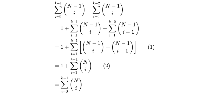
$$ \sum_{i=0}^{k-1}{\binom{N}{i}}=\sum_{i=0}^{k-1}{\binom{N-1}{i}}+\sum_{i=0}^{k-2}{\binom{N-1}{i}} $$

Steps:

$$ \begin{align} &\sum_{i=0}^{k-1}{\binom{N-1}{i}}+\sum_{i=0}^{k-2}{\binom{N-1}{i}} \nonumber \\ &=1 + \sum_{i=1}^{k-1}{\binom{N-1}{i}}+\sum_{i=1}^{k-2}{\binom{N-1}{i-1}} \nonumber \\ &=1 + \sum_{i=1}^{k-1}{\left[\binom{N-1}{i}+\binom{N-1}{i-1}\right]} \qquad\text{(1)} \nonumber \\ &=1 + \sum_{i=1}^{k-1}{\binom{N}{i}} \qquad\text{(2)} \nonumber \\ &=\sum_{i=0}^{k-1}{\binom{N}{i}} \nonumber \end{align} $$

Note: An intuitive way to understand how (1) becomes to (2) is to consider the essence of the combination formula. The term $\binom{N}{i}$ represents the number of ways to choose $i$ people from a total of $N$. There are two mutually exclusive scenarios for any particular person: either they are chosen, or they are not.

If the person is not chosen, then we need to select all $i$ people from the remaining $N-1$, giving $\binom{N-1}{i}$ combinations. If the person is chosen, we have already selected one, so we only need to choose the remaining $i-1$ people from the other $N-1$, resulting in $\binom{N-1}{i-1}$ combinations. Together, these two cases account for all possible selections.